Interaction of household income, consumption and wealth - statistics on main results

Data extracted in March 2023

Planned article update: September 2024

Poverty indicators purely based on income statistics do not reflect the full picture of a household’s economic vulnerability. Consumption and wealth are two additional key dimensions that determine the economic opportunities of people or material inequalities. By merging the three dimensions income, consumption and wealth (ICW) into one dataset, an analysis of the joint distribution of these dimensions can be made by building a number of ad hoc indicators for European Union countries. These indicators can help answer questions such as: Which part of the population is vulnerable in more than one dimension? Which characteristics do vulnerable households expose?

This article presents experimental results drawn from the joint distribution of household income, consumption and wealth. It should be noted, however, that the joint dataset relies on the statistical matching of various surveys and is therefore based on strong assumptions (see Statistics Explained article on methodological issues). Reference years are 'around 2010' and 'around 2015'^[1]. ICW statistics for Italy and for the Netherlands 2010 are not available due to partly missing expenditure data.

Full article

Income, consumption and wealth indicators

Income poverty in the EU

The EU statistics on income and living conditions (EU-SILC) are the basis of classic poverty indicators. As such, poverty analysis in Europe looks at:

monetary poverty on the basis of the income-based 'at-risk-of-poverty' (AROP) indicator:17.3 % of individuals living in the EU-27 were at risk of poverty in 2015 (17.1 % in 2018) [ilc_li02].
severe material deprivation which affected 8.4 % of the population in the EU-27 in 2015 (6.1 % in 2018) [ilc_mddd11]; and
very low intensity work which concerned 10.7 % of the population aged 0-59 in the EU-27 in 2015 (8.8 % in 2018) [ilc_lvhl11].

Because poverty reduction is an important European and global objective, these indicators are studied very carefully (see Income poverty statistics). The ‘at-risk-of-poverty-or-social-exclusion’ (AROPE) indicator, which is the headline indicator to monitor poverty in the EU, combines the three concepts above: 23.8 % of the population in the EU-27 were at risk of poverty or social exclusion in 2015 (21.9 % in 2018) [ilc_peps01].

Low levels of expenditure

Like income, consumption can also be used as a criterion for defining who is a 'vulnerable individual'. Vulnerability can be determined on the basis of consumption expenditures ^[2] rather than household disposable income, with equivalised expenditures replacing equivalised income. Consequently, people with equivalised expenditures below 60 % of the median equivalised expenditures are considered as suffering from low levels of expenditure^[3]. The figures can then be compared based on disposable income and those based on expenditures (see Figure 1). The at-risk-of-poverty thresholds for income can be found here for each country.

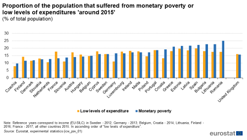
Figure 1: Proportion of the population that suffered from monetary poverty or low levels of expenditures 'around 2015'. (icw_pov_01)

In many countries, the proportion of individuals suffering from low levels of expenditure is very similar to the proportion of individuals below the income-based AROP threshold. In some countries, however, using the expenditure approach may change the conclusions arrived at. For instance, in countries such as as Germany, Bulgaria and Romania, the proportion of persons with equivalised income under the AROP was significantly higher than the rate of persons living with levels of expenditure under the threshold in 2015. Certainly, consumption expenditures fluctuate less over time than income and might therefore be a more stable indicator.

Asset-based vulnerability

A third poverty aspect consists of the accumulated wealth held, or not, by a household. Households tend to accumulate wealth as a precaution, using their assets as a buffer for smoothing out variations in income over time. As such, 'households at risk of asset-based vulnerability' are defined as those households whose total assets do not enable its members to stay above the AROP threshold (60 % of median equivalised income) for longer than a given period of time. In other words, in the hypothetical event of the household ceasing to receive income, its wealth (used to finance the needs of its members) will be used up almost entirely after a period of x months.

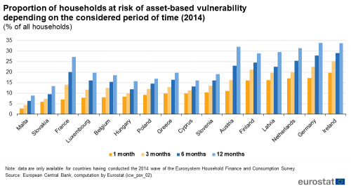
Figure 2: Proportion of households at risk of asset-based vulnerability depending on the considered period of time. (icw_pov_02)

The countries with the highest rates of households at risk of asset-based vulnerability are not the same as those with the highest AROP rates: In Ireland, Germany, the Netherlands, Latvia and Finland more than 15 % of the households were at risk of asset-based vulnerability (after one month) in 2014, which means that they would fall below the income poverty threshold after only one month without income (Figure 2^[4]). The countries with the lowest rates of asset-based vulnerability are those with the highest rate of home-ownership. This illustrates one of the main drawbacks of this indicator: the wealth concept is not based on liquid assets alone, but includes valuables and real estate property. Thus, the indicator will result almost systematically in home-owners not being among the 'vulnerable', despite the difficulties they may encounter to sell their real-estate assets to finance consumption needs. Nevertheless, home-owners do benefit implicitly from an additional source of income, as they use their home for housing, as if they were landlord and tenant at the same time. National accounts have introduced imputed rents precisely to account for this source of income. Also at the micro-level, some experiments have sought to account for this implicit income^[5].

Saving disparities

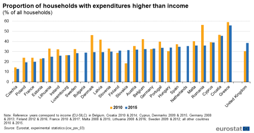
Figure 3: Proportion of households with expenditure higher than income (icw_pov_03).

In order to understand the dynamics of wealth inequality, it is essential to describe the process of asset accumulation and therefore saving behaviours. Saving flows may be defined as the residual between income and consumption, i.e. what is left from income at the end of the period after expenditures for consumption. If income is higher than consumption, this residual is invested in (financial or real) assets and will constitute a part of the wealth held by the household. If consumption is higher than income, the household will have to finance its consumption not only from income, but also by contracting debt or selling assets.

The fact that a household cannot finance its consumption entirely from its income may be a good indication of financial difficulties. As shown in Figure 3, the proportion of households whose yearly expenditures are higher than their income (‘dissaving households’) varies greatly across countries, although this indicator has to be interpreted with caution, as it may be affected by significant measurement errors.

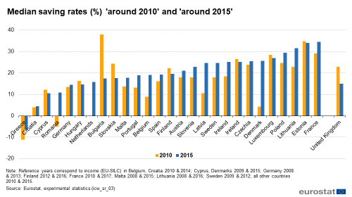
Similarly, a saving rate of close to zero suggests that the household is unable to save and is more likely to restrict its expenditures, thereby not meeting all its needs. Saving rates are computed by dividing savings (the difference between total disposable income and total consumption at the end of year X) by the total disposable income of the household during the same year. The median household saving rate (when households are ranked according to their saving rates, half are above this rate and half are below) can be looked at as another distributional indicator. In 2015, for example, half of all households in Austria were able to save at least 21 % of their annual income (up from 18 % in 2010), but the situation of households in Greece was more difficult, as over half could not finance their expenditure from their income (Figure 4).

Figure 4: Median saving rates (%) of households 'around 2010' and 'around 2015'. Source: Eurostat (icw_sr_03)

Inequality in households' income, expenditures, savings and wealth

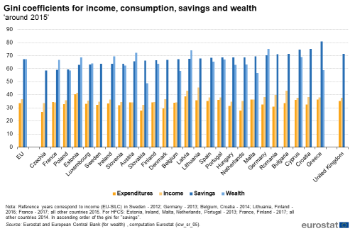
Figure 5: Gini coefficients for income, expenditures, savings and wealth (icw_sr_05)

The gini coefficient is the most common indicator used to express inequality. Wealth is in general far more unevenly distributed than income or consumption. Figure 5 shows the gini coefficients for households' income, expenditures, savings and wealth for European countries in 2015. The coefficients range between 27 and 41 for consumption and between 32 and 46 for income, but they go from 49 to 75 for wealth and even higher for savings.

Interplay between indicators

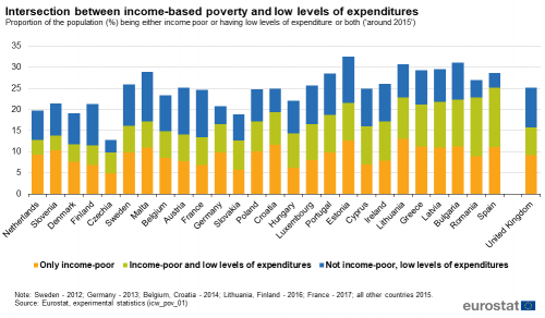
Apart from the accounting exercise of computing savings from income and consumption at household level, it is also interesting to focus on the interplay between the various indicators of vulnerability described above. In particular, individuals who are poor according to the usual income-based definition and at the same time vulnerable with respect to their expenditure levels may be of interest, as they combine several dimensions of poverty. Figure 6 shows the intersection between the usual AROP indicator and the indicator based on consumption; the green segment represents the proportion of the population affected by both types of vulnerability. This proportion is above 10 % for seven Member States (Spain, Croatia, Romania, Greece, Estonia, Latvia and Bulgaria) in 2015. Likewise, it is interesting to observe how the proportion of vulnerable people changes when taking account of consumption. In many countries, more than one person in four is either at risk of poverty due to low income or suffers from low levels of expenditure, in Estonia this applies to almost one in three.

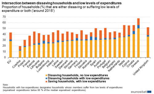
Figure 6: Intersection between income-based poverty and low levels of expenditure 'around 2015' (icw_pov_01) .

By contrast, only a small proportion of households are 'dissaving' and suffer from low levels of expenditure at the same time (see Figure 7), meaning that their consumption does not fall below 60 % of the median consumption of their country although their income does not cover their expenses. In 2015, the highest proportions of households combining the two types of vulnerability were observed in Romania (6.3 %), Greece (5.6 %), Croatia (5.2 %) and Bulgaria (5.0 %).

Figure 7: Intersection between dissaving households and low levels of expenditure 'around 2015' (icw_pov_04).

Consumption expenditures by income

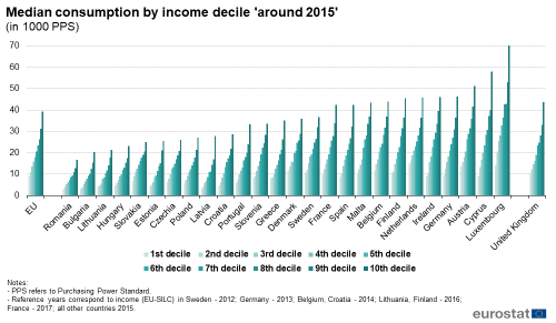
In addition to the indicators above, the joint dataset of households’ income and consumption may be used in a very simple way to show case distributions of median consumption over different income groups (Figure 8). A steep increase in consumption with available income is observed, which is particularly pronounced at the top of the distribution in most countries. The currency purchasing power standard (PPS) makes the distributions comparable among countries, although any country comparison should bear in mind that the statistical matching method relies on different variables for each country and that reference years differ slightly.

Figure 8: Median consumption by income decile 'around 2015', in 1000 Purchasing Power Standard (PPS) (icw_sr_06).

On the other hand, the aggregate prospensity to consume for different income groups can also be displayed.

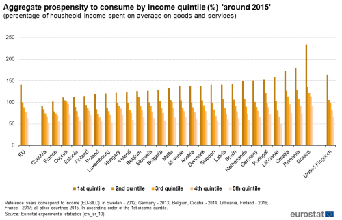
Figure 9: Aggregate prospensity to consume by income quintile (%) 'around 2015' (icw_sr_10).

The aggregate prospensity to consume is defined as the percentage of income spent on average on goods and services. It is derived by using the national accounts approach for the household sector, in which all household income and consumption flows are aggregated at national level. Then, the aggregate consumption expenditure is divided by the aggregate income. The inverse of the aggregate prospensity to consume is the aggregate saving rate, which reflects the saving behaviour of the population as a whole. Figure 9 demonstrates how lower income groups have to spend a considerably higher part of their income on goods and services than higher income groups, thereby preventing them from saving part of their income, or even dissaving as is the case for the first income quintile in almost all EU countries.

Saving behaviours

Understanding households' saving behaviours is relevant for policy-making, as budget choices depend greatly on household characteristics. From this viewpoint, vulnerability may affect different parts of the population, but the essential question relates to the transitory nature of this vulnerability. A household may be able to sustain a low (or even negative) saving rate for a finite period, but people whose expenditures are higher than their income will at some point be confronted with budget constraints.

The role of life cycle

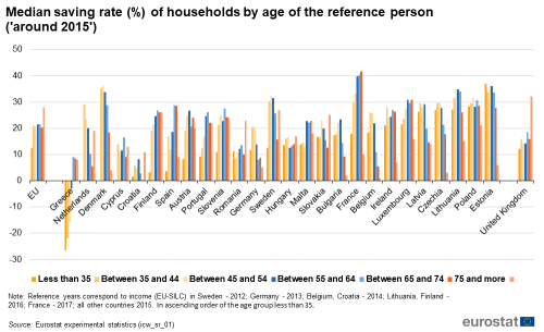
Figure 10: Median saving rate by age of the household reference person 'around 2015' (icw_sr_01)

Economic theory recognises that people's saving behaviour may vary over their lifetime, as they tend to adjust their consumption in order to smooth out income variations. In particular, younger and older people will tend to have lower saving rates, since they are generally earning less than they will earn on average over their lifetime. The data (Figure 10), however, are not conclusive in this regard since there is considerable variation from country to country. Certainly, the age group <35 most often saves less than households whose main earner is older. However, the expected decrease of saving rates after retirement as a result of lower income, for instance, is observed in less than half of the countries (age groups 65+). It is often expected that saving rates will be strongly negative at higher ages, because individuals might want or have to increasingly use up their assets towards the end of their life. This is not corroborated by the data, suggesting that people may retain their assets, in order to pass them on to their children for example.

Household structure and vulnerability

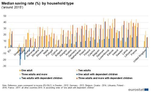
Saving behaviour is also closely linked to household structure (see Figure 11). A family with three children and a single-adult household will have different attitudes to consumption and to the future. As such our data confirm that, in most countries, a lone parent with children is more likely to have a low saving rate. However, the situation varies considerably across Europe and in particular the question whether having children reduces saving rates seems to depend mainly on the social security system in place in the country.

Figure 11: Median saving rate by type of household 'around 2015' (icw_sr_02)

Income and savings

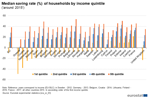
Saving rates increase with income (i.e. the fraction of income not used for consumption increases with income) (see Figure 12). Only five countries show positive median saving rates for the first quintile of income (the 20 % of households with the lowest income): France, Czechia, Ireland, Estonia and Poland. By contrast, Greece (-49.2 %), Croatia (-37.8 %), the Netherlands (-24.5 %) and Romania (-20.6 %), show the most pronounced negative saving rates for households of the lowest income quintile. For Greece and Croatia, even the median household in the second income quintile records a negative saving rate. Solid median saving rates are attained for all countries in the last quintile of income (the 20 % of households with the highest income). The difference in saving rates between the poorest and the richest income quintile is highest (more than 60 percentage points difference) in Croatia, Denmark, Greece, the Netherlands and Lithuania.

Figure 12: Median saving rate of households by income quintile 'around 2015' (icw_sr_03)

Feedback

To help Eurostat improve these experimental statistics, users and researchers are kindly invited to give us their feedback by email

Source data for tables and graphs

Data sources

The annual collection of EU statistics on income and living conditions (EU-SILC) was launched in 2003 and is governed by Regulation 1700/2019 (previously: Regulation (EC) No 1177/2003) of the European Parliament and of the Council. EU-SILC collects information on income and comprises a cross-sectional dimension and a longitudinal dimension. The Household Budget Survey (HBS) is a survey conducted every 5 years on the basis of a gentlemen's agreement between Eurostat, the Member States and the EFTA countries. Data are collected using national questionnaires and, in most cases, expenditure diaries that respondents are asked to keep over a certain period of time. Two waves are used for this article: 2010 and 2015, although the reference year may vary across countries.

Household disposable income is established by adding up all monetary incomes received from any source by all members of the household (including income from work, investment and social benefits) — plus income received at household level — and deducting taxes and social contributions paid. In order to reflect differences in household size and composition, this total is divided by the number of ‘equivalent adults’ using a standard equivalence scale, the so-called ‘modified OECD’ scale, which attributes a weight of 1.0 to the first adult in the household, 0.5 to each subsequent member of the household aged 14 and over, and 0.3 to household members aged less than 14. The resulting figure ('equivalised disposable income') is attributed to each member of the household.

Consumption is described according to the Classification of individual consumption by purpose (COICOP) for each household. Total consumption is obtained by adding up all COICOP items and (as with income) this total is divided by the number of 'equivalent adults' using the same modified OECD scale. The resulting figures are used to compute equivalised expenditures, which are attributed to each member of the household, in order to compute the 'low levels of expenditure' indicator.

EU-SILC and HBS data are matched according to the year of reference for HBS, such as to obtain a fused dataset containing household-level information on both income and consumption. The results are considered valid "around 2010" and “around 2015”. For more details on the statistical matching of EU-SILC and HBS, please see another Statistics Explained article describing the methodology used.

Information on assets and liabilities is from the Household Finance and Consumption Survey (HFCS), in particular the first and second wave conducted in 2010 and 2014. The HFCS is run by National Central Banks and coordinated by the European Central Bank. It collects information on assets, liabilities, and to a limited extent income and consumption, of households. The second wave of the survey is based on 84 000 interviews conducted in 18 euro area countries, as well as Poland and Hungary, mainly in 2013 and 2014.

Context

In order to support its agenda for social fairness and a good balance between economic and social goals, the European Commission has stressed the need to bring social indicators up to a par with macroeconomic indicators within the EU's reinforced macroeconomic governance. To this end, it is important to ensure the availability of harmonised statistics at EU level that cover the distributional aspects of households' income, consumption and wealth (ICW).

In September 2016, the Directorates General of the National Statistical Institutes (DGINS) conference^[6] in Vienna stressed the importance of ICW statistics shedding light on people's material well-being and on inequality. The conference concluded that there was a need for a harmonised statistical framework on ICW based on a multi-source approach integrating existing sources of data (EU-SILC, Household Budget Survey (HBS) and the Household Finance and Consumption Survey (HFCS). These data are the first outcome of data integration effort that will be pursued and improved in the coming years.

In the meantime, Eurostat has launched a section on its website dedicated to the dissemination of experimental statistics. These statistics use new data sources and methods in an effort to expand and improve Eurostat's response to its users' needs. Since the statistics presented in this article come from experimental data processing and are based on statistical assumptions, they belong to this section until they reach a sufficient level of maturity.

Direct access to

Notes

↑ For exact reference years look here.
↑ This is for instance done in the Eurostat publication Monitoring social inclusion in Europe — 2017 edition, pp. 241 - 258.
↑ Consumption or expenditure poverty are alternative terms.
↑ This graph uses data from the Eurosystem Household Finance and Consumption Survey. The HFCS is run by the National Central Banks of the Euro area and coordinated by the European Central Bank. The results published in this article and the related observations and analysis may not correspond to results or analysis of the data producers.
↑ See for instance the Eurostat publication Monitoring social inclusion in Europe — 2017 edition, pp. 141-157.
↑ The DGINS conference is held once a year and aimed at gathering the Directors General of the National Statistical Institutes so as to discuss topics related to the statistical programme. For more details, please have a look here.

[1] For exact reference years look here.

[2] This is for instance done in the Eurostat publication Monitoring social inclusion in Europe — 2017 edition, pp. 241 - 258.

[3] Consumption or expenditure poverty are alternative terms.

[4] This graph uses data from the Eurosystem Household Finance and Consumption Survey. The HFCS is run by the National Central Banks of the Euro area and coordinated by the European Central Bank. The results published in this article and the related observations and analysis may not correspond to results or analysis of the data producers.

[5] See for instance the Eurostat publication Monitoring social inclusion in Europe — 2017 edition, pp. 141-157.

[6] The DGINS conference is held once a year and aimed at gathering the Directors General of the National Statistical Institutes so as to discuss topics related to the statistical programme. For more details, please have a look here.

[1]

[2]

[3]

[4]

[5]

[6]